
Developing Large Power BI Datasets – Part 1
Power BI is architected to consume data in a dimensional model, with narrow fact tables and related dimensions. Introducing a big, wide table in a tabular model is extremely inefficient. It takes up space and memory resources, impacts performance, and complicates measure coding. Flattening records into a flat table is one of the worst things you can do in Power BI and a common mistake made by novice Power BI users.
This is a conversation I’ve had with many customers. We want our cake, and we want to eat it too. We want to have all the analytic capabilities, interactivity and high performance but we also want the ability to drill-down to a lot of details. What if we have a legitimate need to report on transaction details and/or a large table with many columns? It is well-known that the ideal shape is a star schema but what if we need to shape data for detail reporting? The answer is that you can have it both ways, but just not in one table.
For a well-oiled Power BI solution, the following example would be an ideal data model shape:

…but let’s say that for whatever reason, we have a set of requirements that can’t be accomplished using a dimensional model like this. Our skinny fact table doesn’t include all the details and adding them would be very costly. Our requirement is to:
- Drill-down in context, from a summary total to more granular details
- View transactions and detail records
- See recent data changes in real-time
Based on my experimentation, here is an example of the difference in storage efficiency between a star schema and a flat table:
An Import model contains a fact table with 21 million rows. That table has only keys and a few numeric columns. The fact table is related to seven different dimension tables containing unique values and several text-type columns. This PBIX file when fully populated is about 35 megabytes in size. Importing the same data using a TSQL query that joins the fact with same seven dimension tables with repeated attribute values into one big flat table in the Power BI model results in a PBIX file that is about 350 megabytes. So, the same data stored in flat form takes up ten times as much space! Data refresh for the latter model is much slower as well.
DirectQuery and Composite Models
Life is a series of trade-offs and compromises. Adding a DirectQuery table to a model lets you reference an external table from a data source without actually importing the records. Queries against a DQ table are processed at the data source when the user interacts with the report rather than importing a cached copy of the data. When a DQ table is added to a data model with imported tables, it is called a composite model. Import model tables and DirectQuery tables can even have relationships between them. There are many advantages to using this design approach, but the significant trade-off is that DirectQuery typically doesn’t perform well compared to using Import mode tables.
Here is an actual use case:
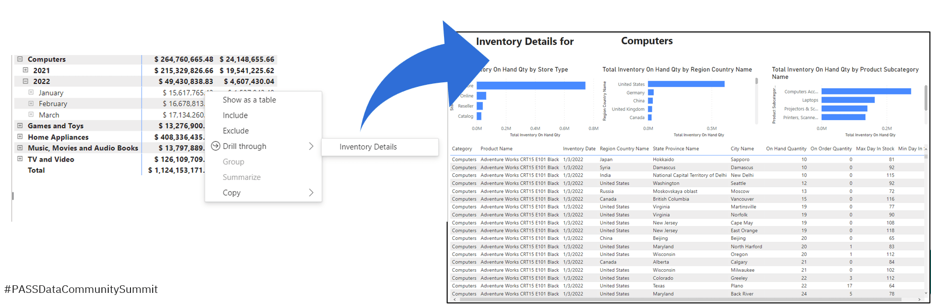
Our details table is imported from an Azure SQL view that contains about 60 columns, many of which are repeating long text values. The table has about 12 million rows and the TSQL script in the underlying view combines several tables using left outer joins. Queries are not fast and can take 30 seconds to a couple of minutes to return results depending on filtering predicates. After adding the table to the model using DirectQuery and adding relationships to common dimension tables, I’ve created a drillthrough report page with parameter fields. There are four visuals on the page that group aggregate values using different fields. When drilling through to the page, filters are passed as parameters to the generated WHERE clause. In one typical test case, the page takes about a minute to render.
The DirectQuery table doesn’t add storage overhead to the model, but users aren’t very happy waiting a minute or more to see results.
Using Aggregations
To design aggregations, you create a table that contains the summarized and aggregated values at levels anticipated from common report grouping. The aggregation design creates a mapping between the detail and summary tables that will be used when a report user navigates to a level supported by the summary table.
I add a new table to the model called Sales Agg that contains only five columns: three keys and two summarized numeric fields. The aggregation design for the summary table looks like this:
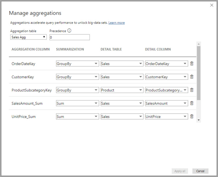
The results are clear. Because the three column charts on the drillthrough report page produce queries supported by the aggregations, those three visuals render in about a second. The table visual isn’t supported by aggregations so it still takes several seconds to render – although less time than before because there was no competition for resources after the first three queries had completed. This at least gives the users summary results to read as they are waiting for the details table.
Troubleshooting and Optimizing Aggregations
The first time I tried to use the aggregations in the chart that grouped by the Region Country Name field, performance didn’t improve, so I knew that something was wrong. To troubleshoot, I captured the generated DAX query using Performance Analyzer, pasted it into DAX Studio and ran a trace using Server Timings. The Server Timings trace revealed that the attempt to use aggregations failed because I had accidentally used the Region Country Name field from the Inventory Details table rather than the Store dimension table referenced in the aggregation design. This was my goof, but it was easy to find and correct using the trace.

Adding a detail table to a model can get messy, especially if the table or view design changes over time. In an effort to keep datasets streamlined and easier to maintain, it may be best to keep the model uncluttered and leave these complicated table out of the Power BI model, just keeping the dimensional star schema.
Drillthrough to a Paginated Report
Paginated reports can report on data in a Power BI dataset but sometimes it’s best to use them for the exceptional reports that are best served using conventional SQL queries. In this example, I have created an Inventory Details report using a TSQL query that delivers the flat, wide detailed results (this is the wide table we were trying to avoid using in the Power BI data model). The reports accepts a few parameters used to filter the query.
Once deployed to the Power BI service, I can execute the Inventory Details report by passing parameter values in the URL.
In my Power BI report, I can build the URL string using a measure used to form a link to the target paginated report. My Inventory Report Link measure is defined using this DAX code:
The measure is categorized as a web link and then can be added to any visual that supports link navigation, in this case the matrix visual.

Here is an example of the link generated by the measure, including the three parameter values related to the selected Category, Year and Month:

A significant advantage is that we are able to use the right reporting tool to server two different purposes. Power BI is great for analytical reporting based on a semantic data model, and Paginated reports is a great tool for detail reporting directly from a transactional database. There is no need to clutter and complicate the data model when I can just use the best tool for the job, and then provide navigation features to make them work together.


While this may be true in the majority of situations – I recently did some testing on import load performance of star schema vs one-big-table “OBT” (or multiple OBT’s in our case) and found the OBT solution to import much faster. I think, this is because our data model is a constellation of star schema’s (fact order, fact order line, fact order line item, fact product + all the dims for each star, this is around 60+ tables). Some of these tables are over 100m rows. We only want to see orders in the past couple of years, and consequently only products associated with those orders, and finally, only dim values that relate to those orders and products in the past couple of years.
Because of this, each fact and (significantly large) dim table needs to first lookup and find the orders sold in the last two years, then use these order id’s as a filter/inner join on each fact and dim to ensure we’re only loading the relevant rows we need. If we do this for all the fact tables, and the larger dimension tables, it means we are querying the fact order table over and over again. Doing the same thing using a few wide tables (one table each for orders, order lines, order line items and products) and doing all the filtering in 4 SQL queries resulted in a much faster import time.
I know that the star schema version will be much smaller in model size, and probably more performant due to the high cardinality of some of the columns, right now we’re more worried about refresh/load speed as our report refreshes kick off about 7am after the nightly ETL has run – so we need these reports to be ready by 9am for the business to consume. I may be missing something obvious here so would appreciate your thoughts on this dilemma.
Note: We can’t utilise incremental refresh because a small portion of our historical data updates very far back in time (over 2+ years), it’s only a few rows per partition, but enough that when we trigger an incremental refresh every single partition has to reload essentially meaning IR = full refresh – hence the concern for refresh/load efficiency.
As always Paul, thanks for your detailed explanations!